ブロック配置のカラフルなポスター

私たちは、たとえば学会や大学・研究機関の壁で見かける情報ポスターや学術ポスターを知っています。

それらには主に次のような共通した特徴があります。

A2、A1、あるいはA0といった大きなサイズであること。
遠くから見ることもあれば、非常に近くから見ることもあること。

その結果、組版にはいくつかの要件が生じます。

ページレイアウトの寸法は、このような大きなサイズに対応している必要があります。
幅広いフォントサイズが必要です。近くに立って読める必要がありますが、同時に目を引く大きな見出しも必要です。
ポスターは読みやすいブロックに分割されているべきです。特に、各ブロックは本文で一般的な行幅を大きく超えないようにする必要があります。行が広すぎると、集中しづらくなり、次の行の先頭に戻るのが難しくなります。そのため、ブロック内の行はおよそ40～50文字程度を大きく超えないようにするのが望ましいです。
各ブロックには明確な見出しが必要です。
色や線などのグラフィック要素を使って、部分ごとに区切ることができます。
画像はベクター形式であるか、高解像度である必要があります。

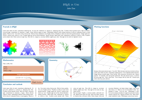
ここでは、A0サイズの横向きポスターを作成します。ダミーテキスト（プレースホルダー）、数式、画像を含むいくつかのブロックを表示します。サンプル画像として、http://texample.net のために作成したフラクタルと、第10章「数式の高度な書き方」にあるプロットおよび幾何図を使用します。本書では画像をファイルとして読み込みましたが、ここでは単一の自己完結型ドキュメントにするため、ポスター文書内ですべて生成します。後でダミーテキストやその他の部分を自分の内容に置き換えることができます。

tikzposterクラスを使用します。文書は列とブロックで構成されています。

プロットのサンプル数を増やせば、より高解像度にできます。フラクタルの次数を上げるとより細かいフラクタルになりますが、その場合は同時にスケーリング係数を下げてください。これはあくまでポスターのデモンストレーションです。

下の「Open in online editor」をクリックすると、この例をOverleafのLaTeXエディターで直接開くことができます。タイムアウトが発生する場合は、フラクタルやプロットのコンパイルに時間がかかりすぎている可能性があります。そのためにサンプル数を低めに設定しました。私がリンクをクリックした際にはOverleafで正常にコンパイルされました。

コードの解説は『LaTeXクックブック』第1章「ドキュメントクラス」の「レシピ8 大型ポスターの作成」に掲載されています。プロットと幾何図の説明は第10章「Advanced Mathematics」にあり、このギャラリーでもご覧いただけます。

お好みで編集してコンパイルしてください。

% Poster with TikZ
\documentclass[landscape]{tikzposter}
\usetheme{Wave}
\usepackage{pgfplots}% for the 3D plot
\usepackage{tkz-euclide}% for geometry
\usepackage{lipsum}% for dummy text
\usepackage{multicol}% for multiple columns
\usetikzlibrary{lindenmayersystems,shadings}% gives us fractals
\pgfdeclarelindenmayersystem{Koch curve}{
  \rule{F -> F-F++F-F}}
\pgfdeclarelindenmayersystem{Sierpinski triangle}{
  \rule{F -> G-F-G}
  \rule{G -> F+G+F}}
\pgfdeclarelindenmayersystem{Fractal plant}{
  \rule{X -> F-[[X]+X]+F[+FX]-X}
  \rule{F -> FF}}
\pgfdeclarelindenmayersystem{Hilbert curve}{
  \rule{L -> +RF-LFL-FR+}
  \rule{R -> -LF+RFR+FL-}}
\setlength{\columnsep}{4cm}
\setlength{\columnseprule}{1mm}
\newcommand*{\image}[2][]{% For conveniently including images
  \begin{tikzfigure}[#1]
    \includegraphics[width=\linewidth]{#2}
   \end{tikzfigure}}
\usepackage{lmodern}
\renewcommand*{\familydefault}{\sfdefault}% Let's have a sans serif font
\begin{document}
\title{\LaTeX\ in Use}
\author{John Doe}
\maketitle
\begin{columns}
  \column{.65}
  \block{Fractals in \LaTeX}{
    \lipsum[1]
    %\image[\LaTeX\ workflow]{flowchart}% if external
    \tikz\shadedraw[shading=color wheel,scale=2] 
      [l-system={Koch curve, step=2pt, angle=60, axiom=F++F++F, order=4}]
        lindenmayer system -- cycle;\hfill
    \tikz\shadedraw [top color=white, bottom color=blue!80,scale=1.5,
      draw=blue!80!black] [l-system={Sierpinski triangle, step=2pt,
      angle=60, axiom=F, order=8}] lindenmayer system -- cycle;\hfill
    \tikz\shadedraw [bottom color=white, top color=red!80,scale=1.5,
      draw=red!80!black][l-system={Hilbert curve, axiom=L, order=5,
      step=8pt, angle=90}] lindenmayer system; \hfill
    \tikz\draw [green!50!black, rotate=90,scale=1]
      [l-system={Fractal plant, axiom=X, order=6, step=2pt, angle=25}]
      lindenmayer system;\hfill
    \tikz\shade[shading=Mandelbrot set] (0,0) rectangle (15,15);
  }
  \begin{subcolumns}
    \subcolumn{.5}
    \block{Mathematics}{
      Take a coffee, then:
      \vspace{1.4cm}
      \coloredbox{\begin{itemize}
        \item State
        \item Proof
        \item Write in \LaTeX
      \end{itemize}}
      \vspace{1.4cm}
      \innerblock{Integral approximation}{
        \[
          \int_a^b f(x) dx \approx (b-a)
            \sum_{i=0}^n w_i f(x_i)
        \]
      }
    }
    \note[targetoffsetx = 4.5cm, targetoffsety = -5cm,
      angle = -30, connection, width=10cm]{\Large Weight function}
    \subcolumn{.5}
    \block{Geometry}{
    \vspace{-3cm}
    \centering
    \begin{tikzpicture}[scale=1.8]
      \tkzDefPoint(0,0){A}
      \tkzDefPoint(4,1){B}
      \tkzInterCC(A,B)(B,A)
      \tkzGetPoints{C}{D}
      \tkzDrawPolygon(A,B,C)
      \tkzDrawPoints(A,B,C,D)
      \tkzLabelPoints[below left](A)
      \tkzLabelPoints(B,D)
      \tkzLabelPoint[above](C){$C$}
      \tkzDrawCircle[dotted](A,B)
      \tkzDrawCircle[dotted](B,A)
      \tkzCompass[color=red, very thick](A,C)
      \tkzCompass[color=red, very thick](B,C)
      \tkzCompass[color=red, very thick](A,D)
      \tkzCompass[color=red, very thick](B,D)
      \tkzDrawArc[fill=blue!10,thick](A,B)(C)
      \tkzDrawArc[fill=blue!10,thick](B,C)(A)
      \tkzDrawArc[fill=blue!10,thick](C,A)(B)
      \tkzInterLC(A,B)(B,A)
      \tkzGetPoints{F}{E}
      \tkzDrawPoints(E)
      \tkzLabelPoints(E)
      \tkzDrawPolygon(A,E,D)
      \tkzMarkAngles[fill=yellow,opacity=0.5](D,A,E A,E,D)
      \tkzMarkRightAngle[size=0.65,fill=red,opacity=0.5](A,D,E)
      \tkzLabelAngle[pos=0.7](D,A,E){\small$\alpha$}
      \tkzLabelAngle[pos=0.8](A,E,D){\small$\beta$}
      \tkzLabelAngle[pos=0.5,xshift=-1.4mm](A,D,D){\small$90^\circ$}
      \tkzLabelSegment[below=0.6cm,align=center,font=\small](A,B){Reuleaux\\triangle}
      \tkzLabelSegment[above right,sloped,font=\small](A,E){hypotenuse}
      \tkzLabelSegment[below,sloped,font=\small](D,E){opposite}
      \tkzLabelSegment[below,sloped,font=\small](A,D){adjacent}
      \tkzLabelSegment[below right=4cm,font=\small](A,E){Thales circle}
    \end{tikzpicture}    
  }
  \end{subcolumns}
  \column{.35}
  \block{Plotting functions}{
    %\image{plot}% if you would like to include an external image
    \pgfplotsset{width=\linewidth}
    \begin{tikzpicture}
      \begin{axis} [
        title = {$f(x,y) = \sin(x)\sin(y)$},
        xtick = {0,90,...,360},
        ytick = {90,180,...,360},
        xlabel = $x$, ylabel = $y$,
        ticklabel style = {font = \scriptsize},
        grid
      ]
      \addplot3 [surf, domain=0:360, samples=30] 
        { sin(x)*sin(y) };
      \end{axis}
    \end{tikzpicture}
    \lipsum[4]
  }
\end{columns}
\block{Conclusion and outlook}{
  \begin{multicols}{4}
    \lipsum[1-2]
  \end{multicols}
}
\end{document}

ダウンロードはこちら： poster.tex • poster.pdf
Overleafで開く： poster.tex

【新刊案内】『TikZによるLaTeXグラフィックス』

文書から生成されたワードクラウド

3 次元表面グラフ

ブロック配置のカラフルなポスター